

If you’re looking for rising trends on Google, you should extract the data from Google Trends. How to scrape Google Trends data? Scraping data from Google Trends allows you to identify the top search queries on Google Search. This includes the latest insights on Google News, Google Images, Google Shopping, and YouTube.
In this web scraping tutorial, we’ll teach you how to build a simple Google Trends scraper using PyTrends, an unofficial Google Trends API. Don’t worry, we’ll guide you step by step.
And if you’re not comfortable extracting Google Trends data with PyTrends, we also offer an alternative to aggregate Google Trends data using Fetch and Cheerio.
Why Scrape Google Trends Data Instead of Using the Tool Directly?
Before we show you how to extract Google Trends data, let’s discuss why we recommend scraping the data in bulk rather than accessing it directly on the platform.
Extracting Google Trends data in bulk offers significant time and efficiency advantages, allowing you to access millions of datasets effortlessly. While manually requesting data for individual keywords is feasible for smaller lists, it becomes impractical when dealing with hundreds of keywords.
Automating this process using PyTrends, a Python API, streamlines the task and significantly reduces time consumption. Before diving into the code, it’s essential to grasp the underlying principles of Google Trends data extraction.
How Does Google Trends Work?
Google Trends is a tool that represents, well, trends. It does not show any search volume for the keywords.
Instead, it shows these trends in a graph that’s scaled based on the highest peak of interest over the time period we specify.
As an example, let’s look for ‘fidget spinner’ in the US:
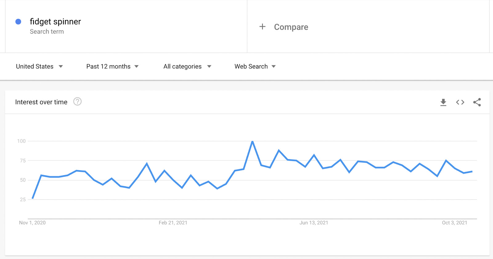
According to the graph, the interest in fidget spinners has been constant and quite high, right? Well… that’s when it gets tricky.
We have to remember that the graph is showing us data based on the highest point over 12 months. 100 represents the highest point and 0 represents the lack of data.
Let’s see what happens when we zoom out:
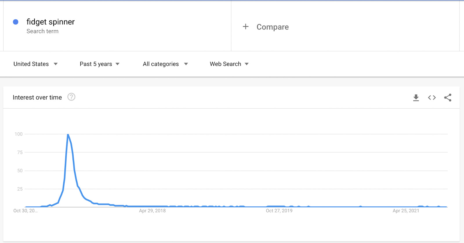
Doesn’t seem so stable now, does it? As we can see, after getting into the market, fidget spinners exploded in popularity and then rapidly decreased in popularity.
Besides timeframe, region, categories and platform will influence the trends data, so make sure to understand what you’re looking for before doing any analysis. So we’ll have to account for those factors in our scraper.
How to Build a Google Trends Scraper with PyTrends
Now that we know the basics let’s start writing our PyTrends Script for how to scrape Google Trends data:
1. Install Python and PyTrends
If you’re using Mac, you probably already have a version of Python installed on your machine. To check if that’s the case, enter python -v into your terminal.
For those of you who don’t have any version of python installed or want to upgrade, we recommend using Homebrew, instructions are inside the link.
With Homebrew package manager installed, you can now install the latest version of Python by using the command brew install python3. You’ll be able to verify the installation with python3 --version command.
The next step is to install PyTrends using pip install pytrends. If you don’t have pip installed on your machine, Python can now install it without any extra tool. Just go to your terminal and type sudo -H python -m ensurepip.
Your development environment should be ready to go now!
Note: when we check the documentation for PyTrends, it says that it requires Requests, LXML, and Pandas. If you don’t have those, just pip install them as well.
2. Connect to Google Trends Using PyTrends
Alright, we’ll create a new file named ‘gtrends-scraper.py’ and open it in your text editor and we’ll add our first lines to connect to Google Trends.
</p>
<pre>from pytrends.request import TrendReq

pytrends = TrendReq(hl='en-US')</pre>
<p>
Note: hl stands for ‘host language’ and it can be changed for any other location you might need.
3. Write the Payload
The payload is where we’ll store all the parameters of our request to be sent to the server. When checking PyTrend’s documentation, we can see there are five different inputs we can add to our payload (which are the same as we would use on the original platform).
- kw_list (list of keywords we want to analyze)
- cat (category)
- timeframe
- geo (region or location of the data)
- gprop (Google’s property)
Let’s take a look at the snippet presented for us in the documentation:
</p>
<pre>kw_list = ["Blockchain"]

pytrends.build_payload(kw_list, cat=0, timeframe='today 5-y', geo='', gprop='')</pre>
<p>
The cat is equal to 0 as a default. If you go to Google Trends and change the category, you’ll be able to see that every category has a value assigned.
![]()
For example, for ‘Arts & Entertainment’ cat is equal to 3. Depending on your needs, you can change this value to whatever category you want to select. For this example, let’s set it as 14 for ‘People & Society’.
Note: Noticed that although ‘blockchain’ is only one keyword, it is still passed as a list. Also, there’s a limit of 5 keywords we can send at a time but that’s because it’s the same limit of keywords we can compare on Google Trends’ site. But you can add more than 5 to the list as long as you’re passing them one by one.
We’ll add our parameters values as variables to make it easier to work with them. So here’s how our code is looking so far:
</p>
<pre>from pytrends.request import TrendReq

pytrends = TrendReq(hl='en-US')

all_keywords = [
	'event management',
	'event planning',
	'event planner'
]
cat = '14' #people&society
timeframes = [
	'today 5-y',
	'today 12-m',
	'today 3-m',
	'today 1-m'
	]
geo = '' #worldwide
gprop = '' #websearch
pytrends.build_payload(
	kw_list,
	cat,
	timeframes[0],
	geo,
	gprop
)</pre>
<p>- We use a variable named
all_keywordsbecause we’ll use it to pass each keyword individually – if not, it would compare them with each other. - We added a variable for time frames to be able to analyze the keyword from different timeframes. However, the
[0]will select the first one of the list.
3. Extract Data from Google Trends
The first thing we need to implement is a temporary list called keywords and make it an empty list: keywords = []. Then, we’ll wrap our payload inside a function called check_trends().
Plus, we’ll add a new variable to our function that will return pandas.Dataframe: data = pytrends.interest_over_time().
</p>
<pre>keywords = []

def check_trends():
	pytrends.build_payload(
		kw_list,
		cat,
		timeframes[0],
		geo,
		gprop
	)
	data = pytrends.interest_over_time()

for keyword in all_keywords:
	keywords.append(keyword)
	check_trends()
	keywords.pop()</pre>
<p>
The for loop at the end will take a keyword from our main list and append it to our empty list. Then it will pass only that keyword to our check_trends() function for analysis before popping it out, leaving an empty list again, and pushing the next one.
4. Determining If There’s a Trend
Our code as-is will get data from Google Trends and bring it back. However, we’ll need to do further analysis if to interpret the data.
Let’s start by calculating the mean:
</p>
<pre>mean = round(data.mean(),2)

print(keyword + ': ' + str(mean[keyword]))</pre>
<p>
Here’s how the output should look like:
Here’s where understanding the way Google Trends work will pay off. Because we’re reading the mean in a 5 years timeframe, we need to understand that there was a point when the interest overtime was 100, so a low number would mean that over the five years, the interest has been pretty low.
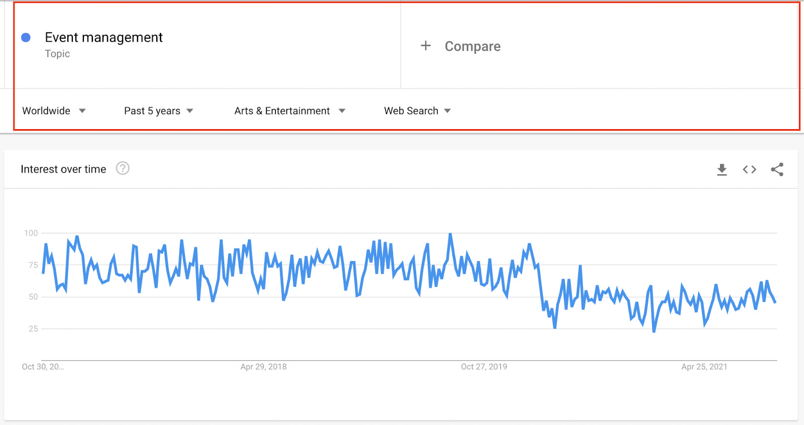
To make it easier to visualize here’s the graph for ‘event management’:
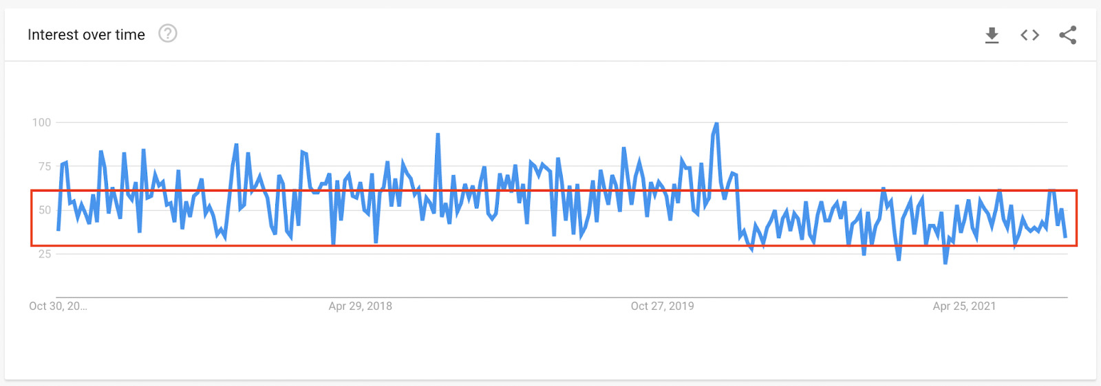
As you can see, over the period of five years, it has stayed pretty stable, with the highest peak being around February 2020. We could read this query as stable but not rising in popularity. So, for a new business, there’s a stable need for event management professionals, services, and software.
Ok, we might need more information to jump to that conclusion, but as you can see, that’s exactly the kind of assumption we can make by using data from Google Trends.
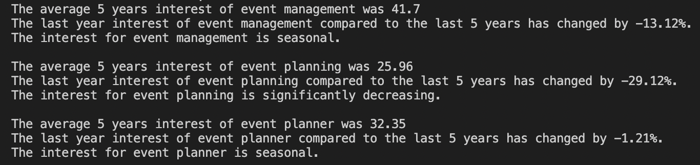
For example, event planning at 25.96 is fairly low in comparison to the peak, so we could conclude that this is a query without much popularity, right? Well, maybe. But remember that this is a mean, it could happen that it is a seasonal query with peaks closer to 100 in specific months.
Automating Conclusions With PyTrends
Here’s an exercise, we want to know how does last year’s trend compares to the rest of the timeframe.
</p>
<pre>avg = round(data[keyword][-52:].mean(),2)

trend = round(((avg/mean[keyword])-1)*100,2)

print('The average 5 years interest of ' + keyword + ' was ' + str(mean[keyword]))

print('The last year interest of ' + keyword + ' compared to the last 5 years has changed by ' + str(trend) + '%.')</pre>
<p>
What we’re doing at this point is calculating the average trend without the last 52 weeks (because Google Trends is sending us weekly data) that would represent the last year and then calculating the change of trend converting it in percentages.
This is how the outcome would look like:
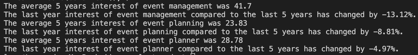
So there’s a new conclusion to be made. Yes, the mean interest of the queries has been fairly stable (spacially for ‘event management’), but the overall interest has been decreasing in the last year.
However, we can automate more conclusions faster using Python than just going through the data by hand. These are a few conclusions (but not the only ones) we could also run:
</p>
<pre>#Stable trend

if mean[keyword] > 75 and abs(trend) <= 5: print('The interest for ' + keyword + ' is stable in the last 5 years.') elif mean[keyword] > 75 and trend > 5:

	print('The interest for ' + keyword + ' is stable and increasing in the last 5 years.')

elif mean[keyword] > 75 and trend < -5: print('The interest for ' + keyword + ' is stable and decreasing in the last 5 years.') #Relatively stable elif mean[keyword] > 60 and abs(trend) <= 15: print('The interest for ' + keyword + ' is relatively stable in the last 5 years.') elif mean[keyword] > 60 and trend > 15:

	print('The interest for ' + keyword + ' is relatively stable and increasing in the last 5 years.')

elif mean[keyword] > 60 and trend < -15: print('The interest for ' + keyword + ' is relatively stable and decreasing in the last 5 years.') #Seasonal elif mean[keyword] > 20 and abs(trend) <= 15: print('The interest for ' + keyword + ' is seasonal.') #New keyword elif mean[keyword] > 20 and trend > 15:

	print('The interest for ' + keyword + ' is trending.')

#Declining keyword

elif mean[keyword] > 20 and trend < -15: print('The interest for ' + keyword + ' is significantly decreasing.') #Cyclinal elif mean[keyword] > 5 and abs(trend) <= 15: print('The interest for ' + keyword + ' is cyclical.') #New elif mean[keyword] > 0 and trend > 15:

	print('The interest for ' + keyword + ' is new and trending.')

#Declining

elif mean[keyword] > 0 and trend < -15:

	print('The interest for ' + keyword + ' is declining and not comparable to its peak.')

#Other

else:

	print('This is something to be checked.')

print('')</pre>
<p>
The power of automating Google Trends with PyTrends is that we can automate as many conclusions as we want, and by changing the list of keywords, we can pull a lot of conclusions with just the press of a button.
Before we say goodbye, we want to show you, fairly quickly, another route you can take to pull trends data using JavaScript this time.
Note: If you want to learn more about Python for web scraping, check our guides on how to scrape multiple pages with Python and Scrapy, and how to build a Beautiful Soup scraper from scratch.
Google Trends Web Scraping Alternative Using Fetch and Cheerio
For this use case, let’s say we want to start a new business but we don’t want to just depend on intuition. We want to create a product that has demand right now.
Setting Up Our Development Environment
To set up our development environment, follow these instructions:
- First, download and install Node.js on your machine: https://nodejs.org/en/download/.
- Next, create a new folder for your project (we’ll use the same we used for our PyTrends project) and navigate to it from your terminal.
- Inside the folder, enter the command
npm init -yto create the necessary files. - To install our dependencies, let’s type
npm install cheerioand thennpm i node-fetch
Pretty simple, right? So let’s move to the next step!
Fetching Our Target URL
Exploding Topics is a relatively new site that analyzes millions of web searches to identify rising (or exploding) queries/topics. This makes it a perfect alternative to Google Trends but the caveat is that we don’t need to analyze the data itself to make conclusions as the website is meant to provide only trending and raising queries.
We’ll change the parameters to ‘1 month’ (to try to catch those new rising topics) and business, and grab the resulting URL ‘https://explodingtopics.com/business-topics-this-month’.
</p>
<pre>import fetch from 'node-fetch';
import { load } from 'cheerio';
(async function() {
	const res = await fetch('https://explodingtopics.com/business-topics-this-month');
	const text = await res.text();</pre>
<p>
Our code is now fetching the URL and then storing the response in the text constant.
That said, there’s one more thing we need to do before parsing the response.
If we want our scraper to scale, we can’t just send all requests through our IP address. Websites will quickly figure out our script isn’t a human and will block it. Making our web scraper useless.
Integrating Fetch with ScraperAPI
For the next step, we want to tell Fetch to send the request through ScraperAPI’s servers. There, it will change the IP address automatically for every request, handle any CAPTCHAs that might get in the way, and use years of statistical analysis to determine the best header to use for the request.
All of this will be handled for us by just adding a few lines to our URL.
First, we’ll create a free ScraperAPI account to generate an API key.
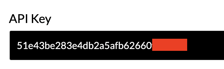
With our API key, we can now build our target URL:
</p>
<pre>const res = await fetch('http://api.scraperapi.com?api_key=51e43be283e4db2a5afb62660xxxxxxx&url=https://explodingtopics.com/business-topics-this-month');</pre>
<p>
Parsing the HTML Response with Cheerio
Now that our scraper is blacklisting-proof, we can send the response to Cheerio for parsing.
First of all, we need to declare Cheerio at the top of our file like this import { load } from 'cheerio' and then add const $ = load(text) to our function.
Done! Our response is now in Cheerio and we can navigate it using CSS selectors.
Let’s say that we want to pull the title, description, and searches per month. For that, let’s grab the bigger element that’s wrapping the elements we’re looking for, a <div> with the class “topicInfoContainer”:
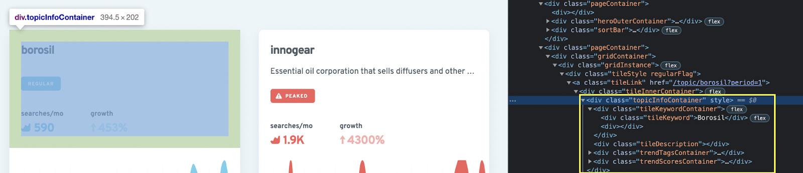
</p>
<pre>const containers = $('.topicInfoContainer').toArray();</pre>
<p>
As you can see, we’re converting the element into an array. It will allow us to select several elements inside the big element we just grab.
Using CSS selectors, we can then get every element inside the Array.
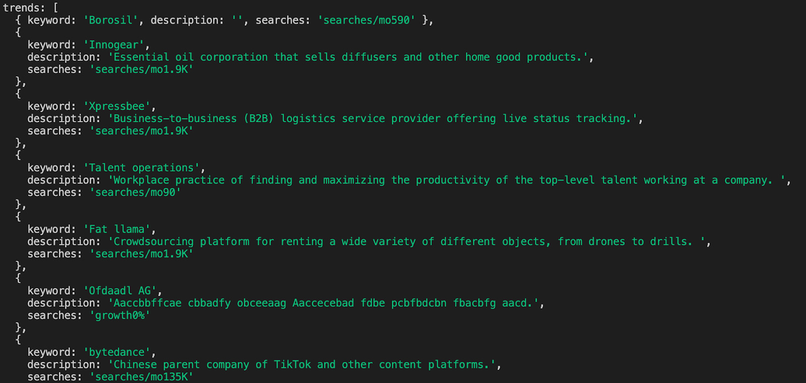
For the sake of simplicity and time, here’s the finished code:
</p>
<pre>import fetch from 'node-fetch';

import { load } from 'cheerio';

(async function() {

	const res = await fetch('http://api.scraperapi.com?api_key=51e43be283e4db2a5afb62660xxxxxxx&url=https://explodingtopics.com/business-topics-this-month');

	const text = await res.text();

	const $ = load(text);

	const containers = $('.topicInfoContainer').toArray();

	const trends = containers.map(c => {

		const active = $(c);

		const keyword = active.find('.tileKeyword').text();

		const description = active.find('.tileDescription').text();

		const searches = active.find('.scoreTag').first().text();

		return {keyword, description, searches}

	})

	console.log({trends});

})();</pre>
<p>
If you run this code in your terminal (adding your own API key), the output should look like this:
Note: For a more in-depth guide on using JavaScript for web scraping, check our step-by-step tutorial on building a Node.js web scraper.
Scrape Google Trends Data at Scale with PyTrends
Congratulations! You have now successfully learned how to scrape Google Trends data by building not one but two Google Trends web scrapers that will bring more and better data to your business.
Whether you are using PyTrends to interact with Google Trends and automate conclusions or using Node.js to scrape ‘hot topics’ to find new business opportunities, ScraperAPI is ready to help you scrape the Google Trends without getting blocked by anti-scraping techniques. Plus, if you also regularly extract other Google data (Google Search, Shopping, and News), you can leverage ScraperAPI’s structured data endpoints to help you get clean, JSON format data.
Curious to see how ScraperAPI simplifies web scraping? Sign up now for a 7-day free trial (5,000 API credits).
Until next time, happy scraping!
Other Google web scraping tutorials that may interest you: